CodingBobby / Fractals
On this page you will find a collection of some fractal images I computed on my own.
I was inspired by Pickover’s great book CPCB1 to explore the chaotic maps using self-written code. But I am no expert and if you want to know how this stuff works, you’d be better off reading his book.
Basically, for each pixel in these images, a feedback-loop is run on their coordinates until one of several conditions is fulfilled that causes the loop to halt. Depending on the exact parameters reached when stopping, the computed pixel is coloured differently. These conditional checks are also called convergence-tests of which Pickover introduced three and accidentally found a fourth one because of a bug in his code.2
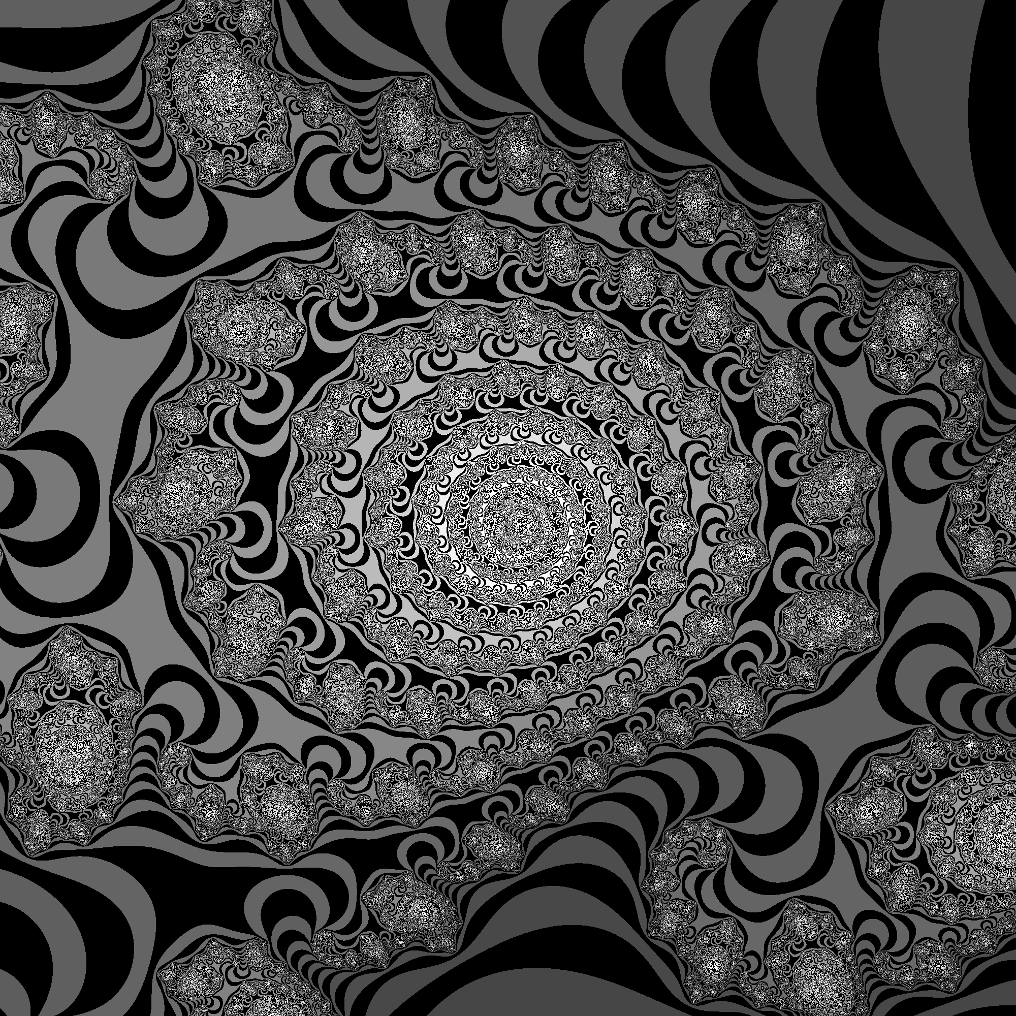
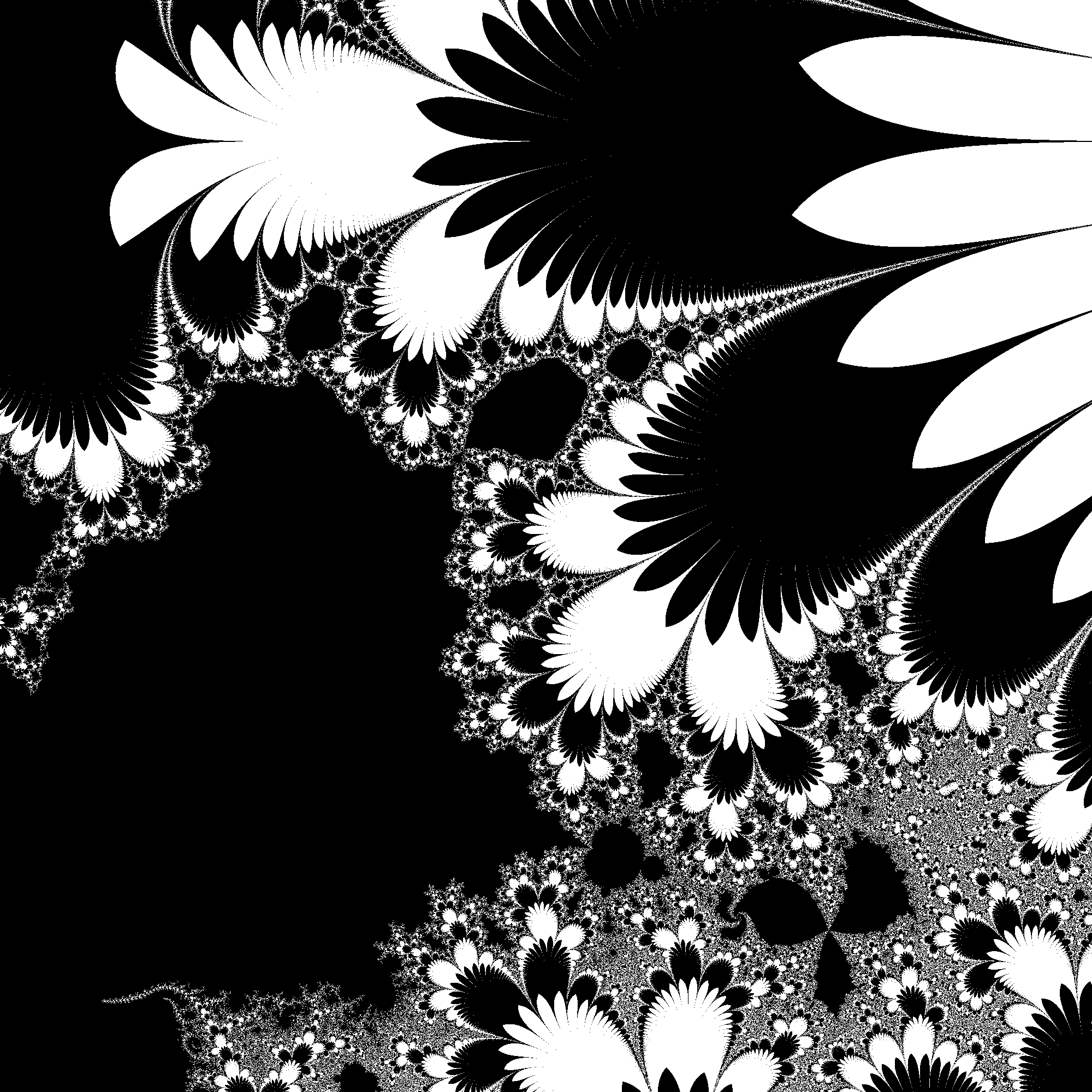
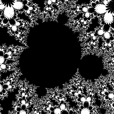
Chaotic Curl
\[f(z) \rightarrow z^2 + \mu\] \[\mu = −0.746 + 0.172\,i\]around \(z_c = 0.046 − 0.849\,i\). Chaotic curls produced with \(70\) iterations and convergence-test \(3\).
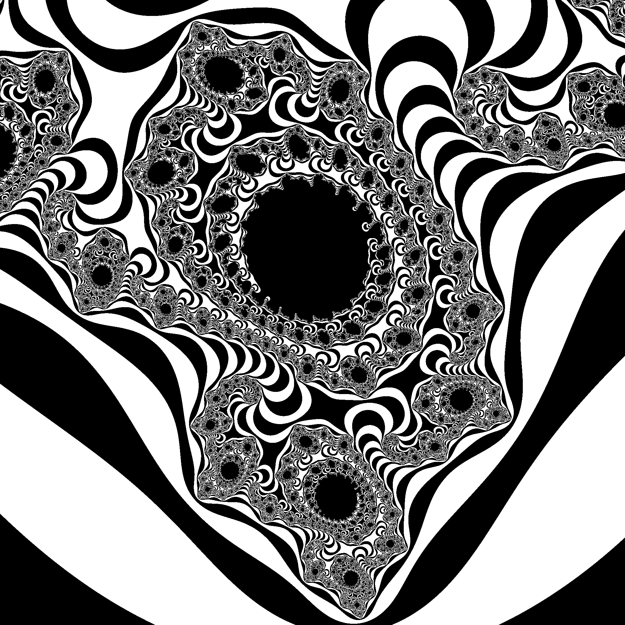
The following one is has its center at \(z_c = −0.1079 + 0.0566\,i\). A maximum of \(400\) iterations were computed with halftone shading to reveal the deep structure of this chaotic curl.
Animated Biomorph
\[f(z) \rightarrow z^z + z^5 + \mu\] \[\mu = −0.746 + b\,i\]The constant \(b\) was animated in the range \(0.00\)–\(1.00\) in steps of \(0.05\) and was shaded using convergence-test \(4\). The center is \(z_c = 0\).
Network
\[f(z) \rightarrow (a + b)^2\] \[a = 2\,z^2\] \[b = 0.176 + 2\,i\]around \(z_c = -0.595 + 0.515\,i\). This organismic fractal is the result of a simple network of adding and squaring. Convergence-test \(4\) was used.
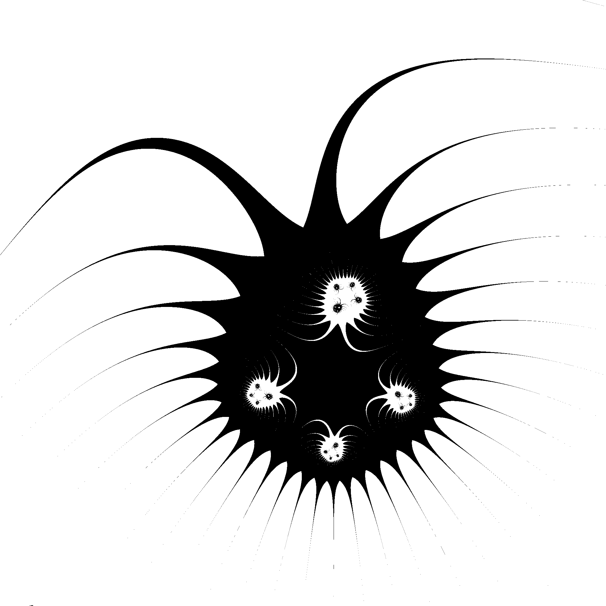
Modifying this network slightly leads to something interesting that reminds me of mitosis of microorganisms:
\[f(z) \rightarrow (a + b)^2 + n\,a\]where \(n\) is animated in the range \(0\)–\(2\) in steps of \(0.1\). The center of the image was adjusted in each frame so that the biomorph doesn’t move as much.
Cosh-Map
\[f(z) \rightarrow \cosh{z} + \mu\]starting with \(z_0 = 0\) around \(\mu_c = 1.12 + 2.4\,i\). Notice the slightly deformed Mandelbrot-Set embedded in the map in the lower middle. Convergence-test \(4\) was used.
A magnification of the embedded M-Set at \(z_c = 1.2565 + 1.8275\,i\):
Convergence-Tests
These are the four tests that were used to compute the images:
\[\sqrt{\Re^2(z) + \Im^2(z)} \leq \tau\] \[\Re(z) \leq \tau \;\wedge\; \Im(z) \leq \tau\] \[\sqrt{\Re^2(z) + \Im^2(z)} \leq \tau \;\wedge\; j \bmod 2 = 0\] \[\Re(z) \leq \tau \;\vee\; \Im(z) \leq \tau\]The constant \(\tau\) is used as a threshold to define when a value is considered to have diverged. For the current number of iterations, \(j\) is used instead of \(i\) to prevent confusion with the imaginary unit.
