The following graphics show the phase space of specific differential systems which contain periodically appearing attractors. Unlike the typical three-dimensional strange attractors, they don’t have a single bounding box no point will ever escape but many more, if not infinitly many covering the entire two-dimensional plane.

These systems can be generally written as

\[\dot{x} = -\,f(y)\] \[\dot{y} = \,f(x)\]

where \(f\) is an arbitrary function dictating the system’s behaviour. Planes are centered at \((0,0)\) unless otherwise stated.

Inspiration for this project was Cliff Pickover’s book CPCB¹ – again, I know; it is like Gabriel’s Horn of chaos for me.

Plane Tesselation

Perhaps the simplest forms \(f\) can take in order to produce a repeating pattern is this:

\[f(u) = \sin(u)\]

And here is the result:

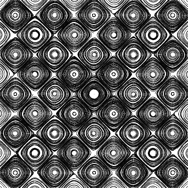
It might already look chaotic but that is mostly because the the sampled points do not align with the pattern. Let’s add another term:

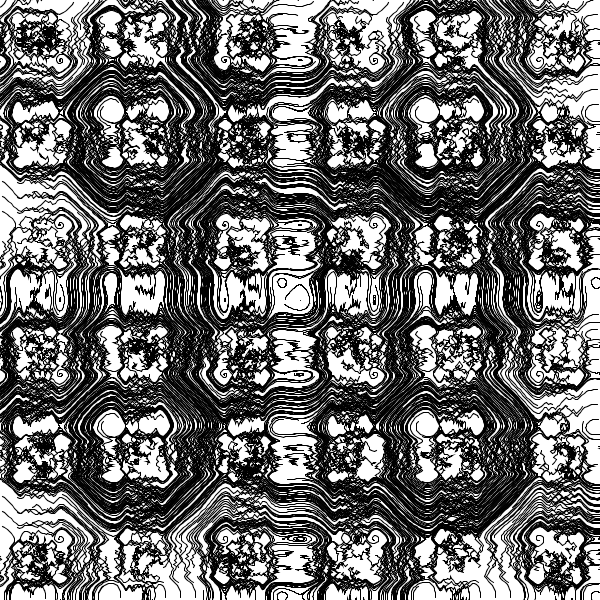
\[f(u) = \sin(u) + \sin^2(u)\]

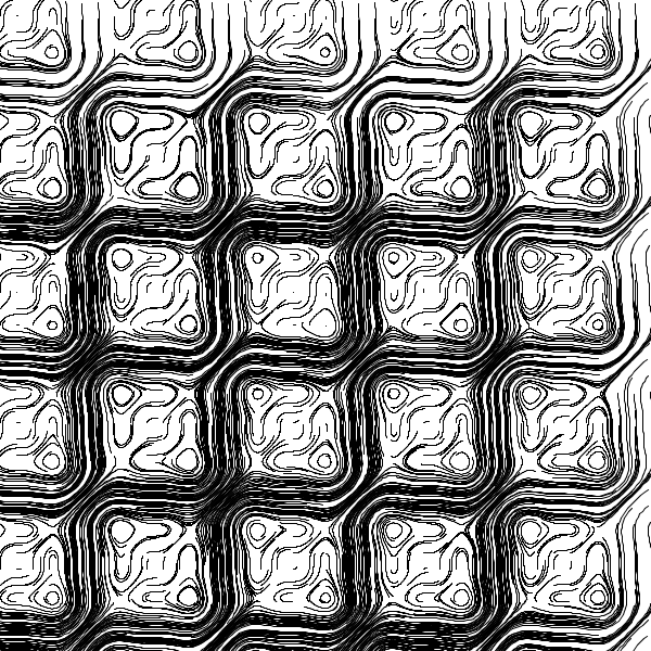
Because these patterns actually get a bit repetitive, I won’t show the following images with the same scale but zoom on more interesting regions. Here, the frequency \(u\) is modulated with another periodic function:

\[f(u) = \sin\left(u + \sin(u)\right)\]

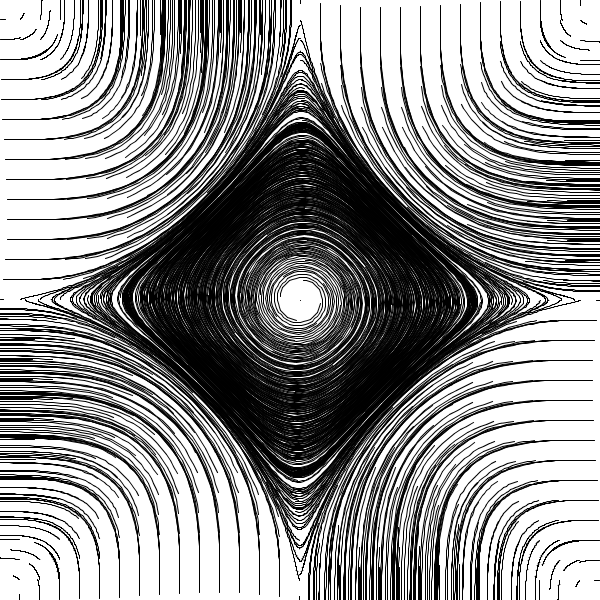
We can change the impact of a specific term or modify its frequency by introducing a factor \(\varrho\):

\[f(u) = \sin\left(u + \sin(\varrho\,u)\right)\] \[\varrho = 5\]

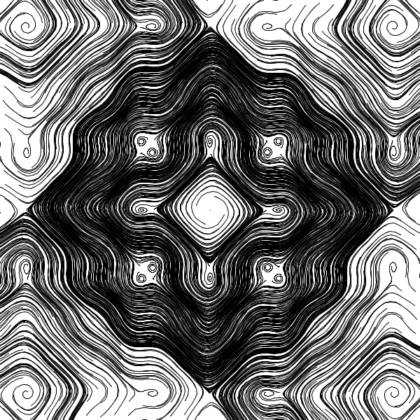
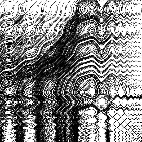
Longer terms allow asymmetric use of \(\varrho\):

\[f(u) = \sin\left(u + \sin^2(\varrho\,u)\right) + \sin\left(\varrho\,u + \sin^2(u)\right)\] \[\varrho = 0.3\]

Even more chaotic behaviour happens with powers:

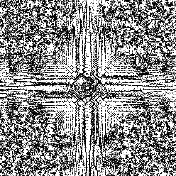
\[f(u) = \sin\left(\varrho^u + \sin^2(\varrho\,u)\right)\] \[\varrho = 3.6\]

Other modulation functions are also interesting. \(\tan\) creates unexpectedly chaotic shapes:

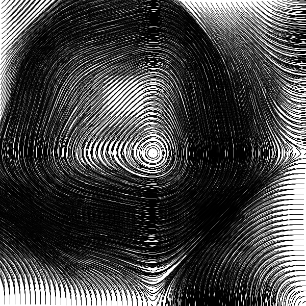
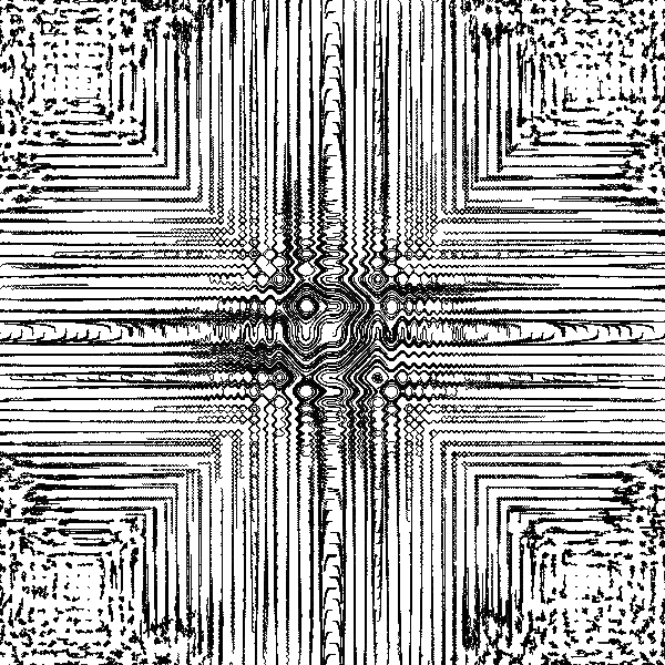
\[f(u) = \sin\left(u + \tan^2(\varrho\,u)\right)\] \[\varrho = 1.5\]

A magnification of the central swirl:

Randomness

Some tesselations get finer and finer towards larger \(x\) and \(y\) until their details hit a limit where the step size \(\dot{x}\) and \(\dot{y}\) respectively is greater than the period of the pattern. Because the points are moving too fast, they overshoot their correct trajectory and get trapped in a neighbouring attractor, which they leave again shortly afterwards. As a result, they walk seemingly randomly across the plane.

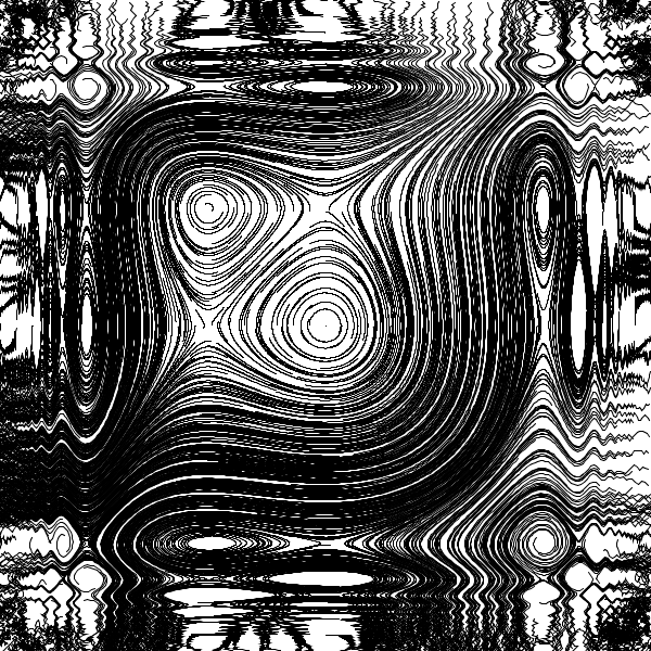
\[f(u) = \sin\left(u^3 + \sin^2(\varrho\,u)\right)\] \[\varrho = 3\]

When the velocity is reduced, the non-random area extends, resolving finer details of the true phase space:

Here is a magnification of the transition between non-random to random walk (in the bottom right quadrant):

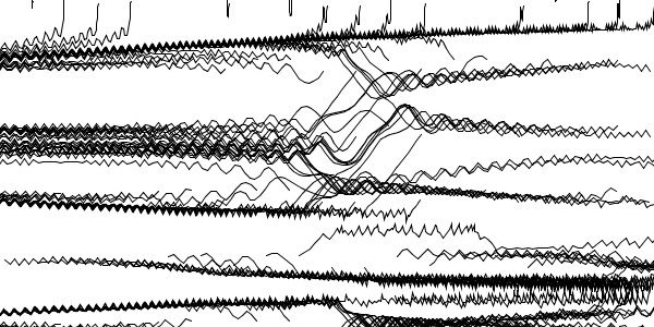
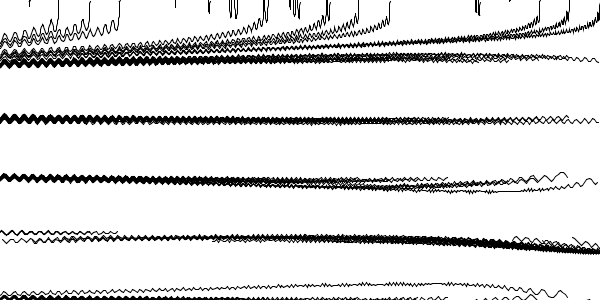
The “moment” when a trajectory is deflected towards another attractor is clearly visible. These are the same points but they are moving with half the velocity (like in the larger images above):

---

1. C.A. Pickover, 1990. "Computers, Pattern, Chaos, and Beauty". St. Martin’s Press. ISBN: 0312041233. ↩