The following graphics show strange attractors, which are different from the typical 3D systems shown in the gallery here. Most importantly, no differential equations are involved; in other words, the initial point doesn’t start to move along a trajectory through 3D space but jumps across a plane in large steps that seem random at first.

Consider this time-discrete system for example:

\[x_{n+1} = \sin(-y_n) - \varrho_n\,\cos(x_n)\] \[y_{n+1} = \varrho_n\,\sin(-1.2\,x_n) - \cos(1.8\,y_n)\] \[\varrho_{n+1} = 0.75\,\sin(x_n)\]

Here is an animation of the first 300 iterations when starting at \((y_0, x_0, \varrho_0) = 0\):

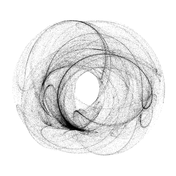
The points indeed seem to appear at random positions; you have no idea where the next one is going to pop up. But at the same time they somehow tend to cluster around a weird shape. This is how it evolves in the long run – one million iterations later to be exact:

You can click on the image to zoom into a version with higher resolution. What you see is an attractor first described by Clifford Pickover in 1988¹ and is thus called the Pickover-attractor or sometimes Clifford-attractor; he later included it in his wonderful book CPCB² where I found it.

The general form of the system is:

\[x_{n+1} = \sin(a\,y_n) - \varrho_n\,\cos(b\,x_n)\] \[y_{n+1} = \varrho_n\,\sin(c\,x_n) - \cos(d\,y_n)\] \[\varrho_{n+1} = e\,\sin(x_n)\]

The variable \(\varrho_n\) could be seen as an extra dimension, but its purpose here is to introduce more randomness to the system that can be controlled with the parameter \(e\). The other parameters \(a\)–\(d\) can be chosen to be any real number. Even slight changes of their values result in very different shapes that seem to share no similarities. Here are some renders I computed for various parameters. Unfortunately I forgot to note them down – because I was so excited to fiddle with them and see the emerging beauty.

More Interesting Systems

There are more such systems found by other people (Henon, Ikeda, de Jong, Juan, Lace, Catrián, etc.), but of course, I have also been searching for equations that would yield chaotic behaviour.

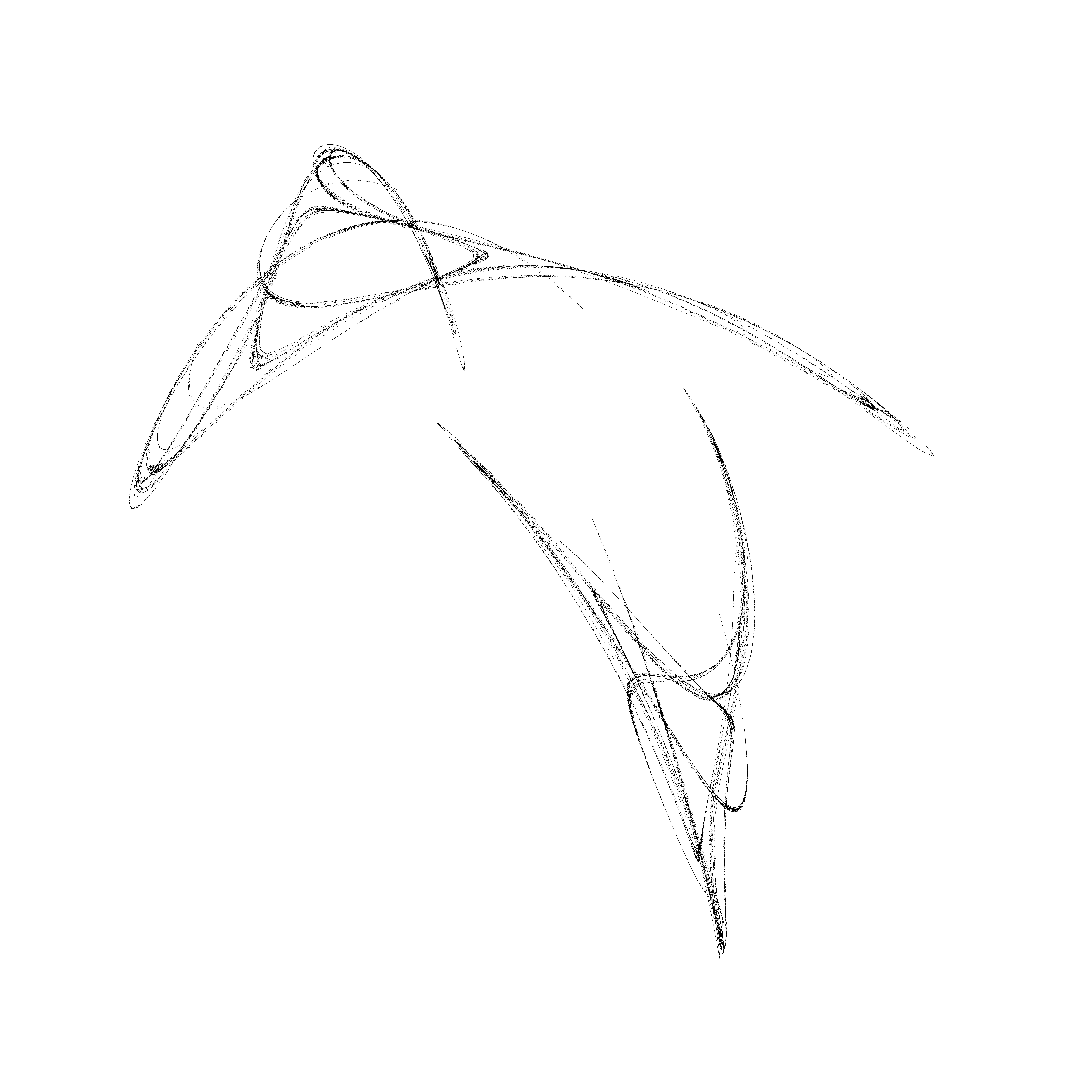
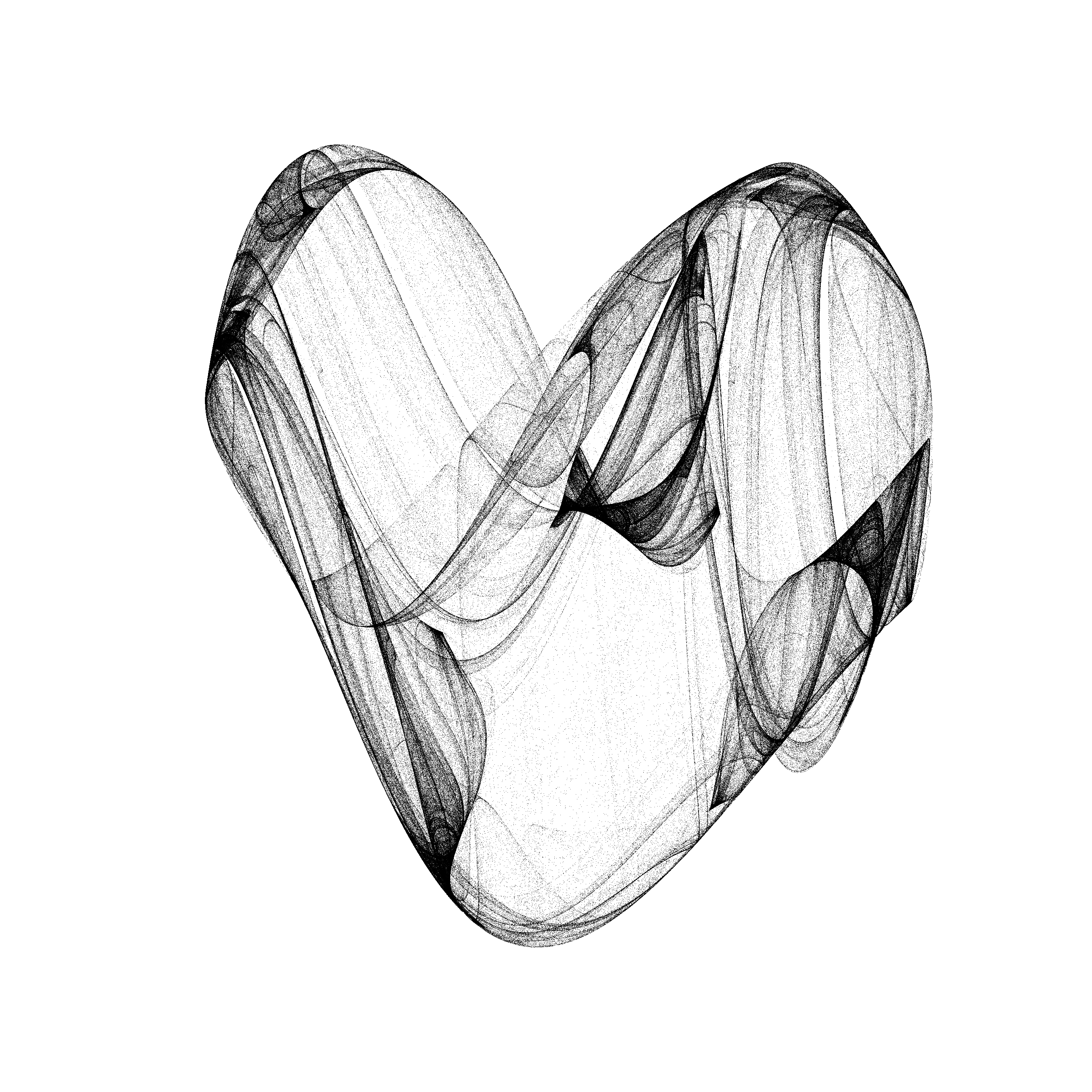
I’m not sure if anyone else has already described it, and although the equations look similar to Pickover’s, they are linearly independent of them. This simple system has just two parameters:

\[x_{n+1} = \sin(a\,y_n) + b\,\sin(a\,x_n)\] \[y_{n+1} = \cos(b\,x_n) + a\,\cos(b\,y_n)\]

Around \(a = 0.838\) and \(b = 2.598\), you will find this wonderful shape – which is why I call it the heart-attractor:

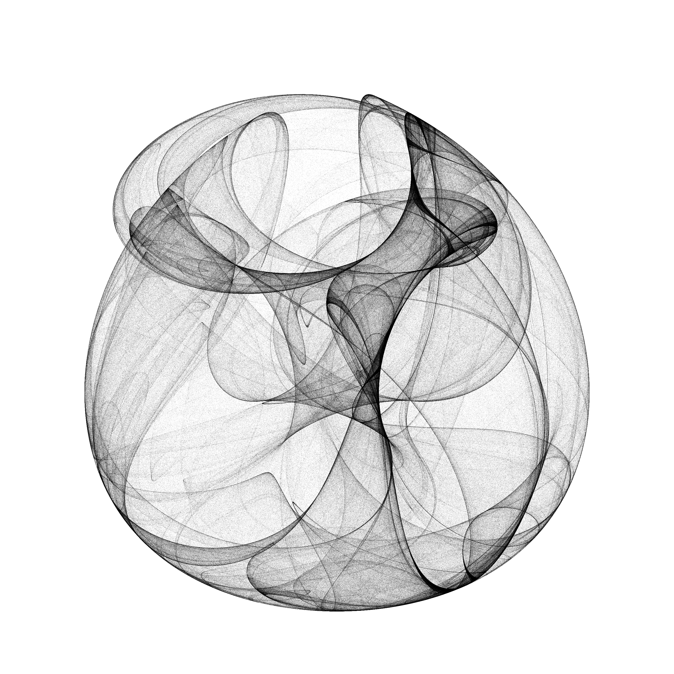
Variating the constants have a great effect on the result; here are some more configurations, like a small bag for picnic:

\[a = 1.605 \,\land\, b = 1.397\]

Or dental roots (I know, I have ultimate imagination):

\[a = 1.728 \,\land\, b = 0.907\]

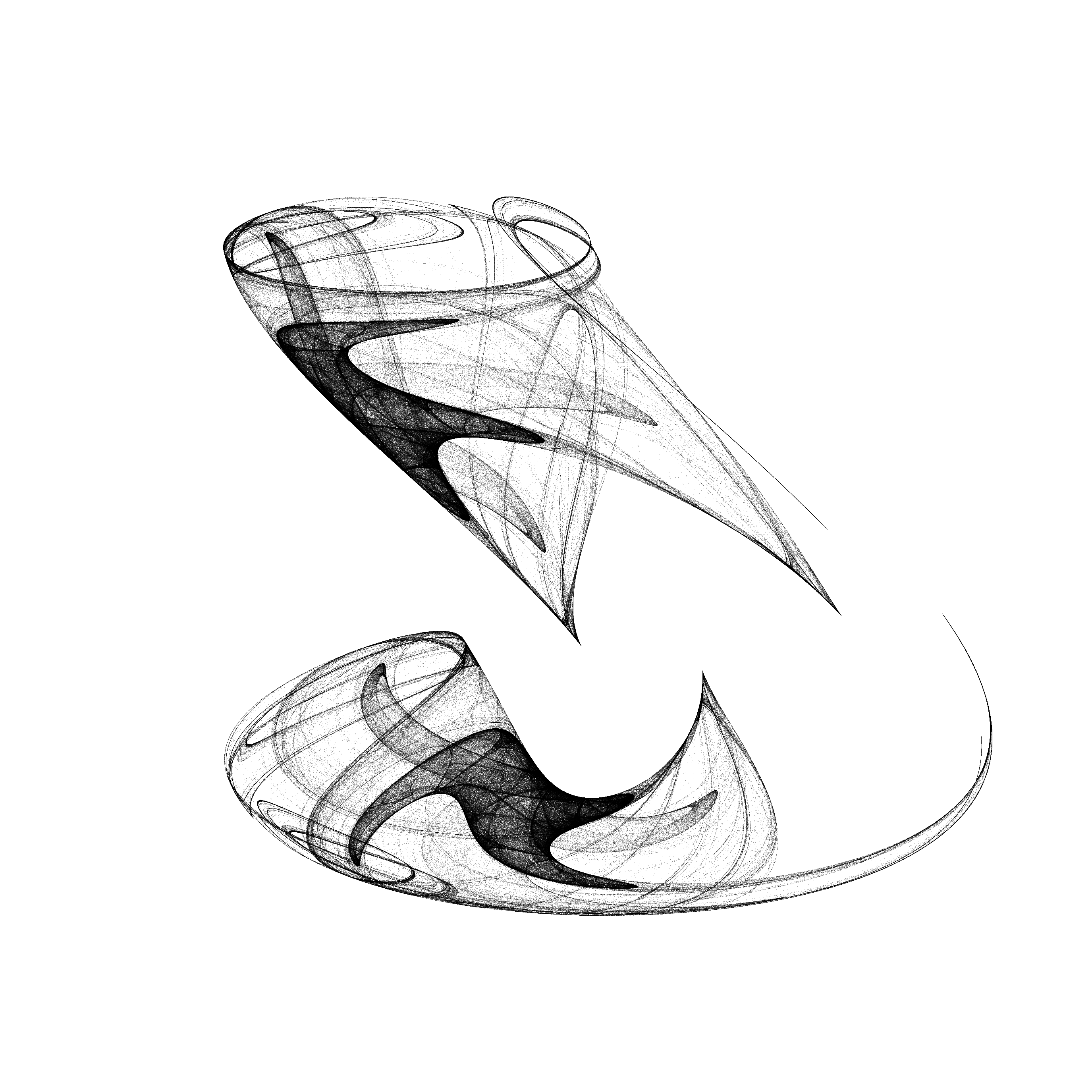
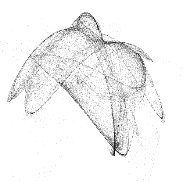
And this curved vase with sinusoidal patterns would look nice in my livingroom:

\[a = 2.479 \,\land\, b = 0.781\]

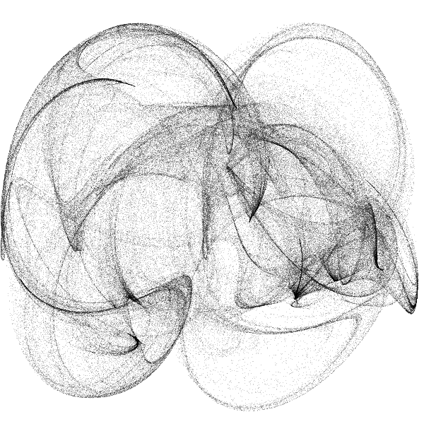
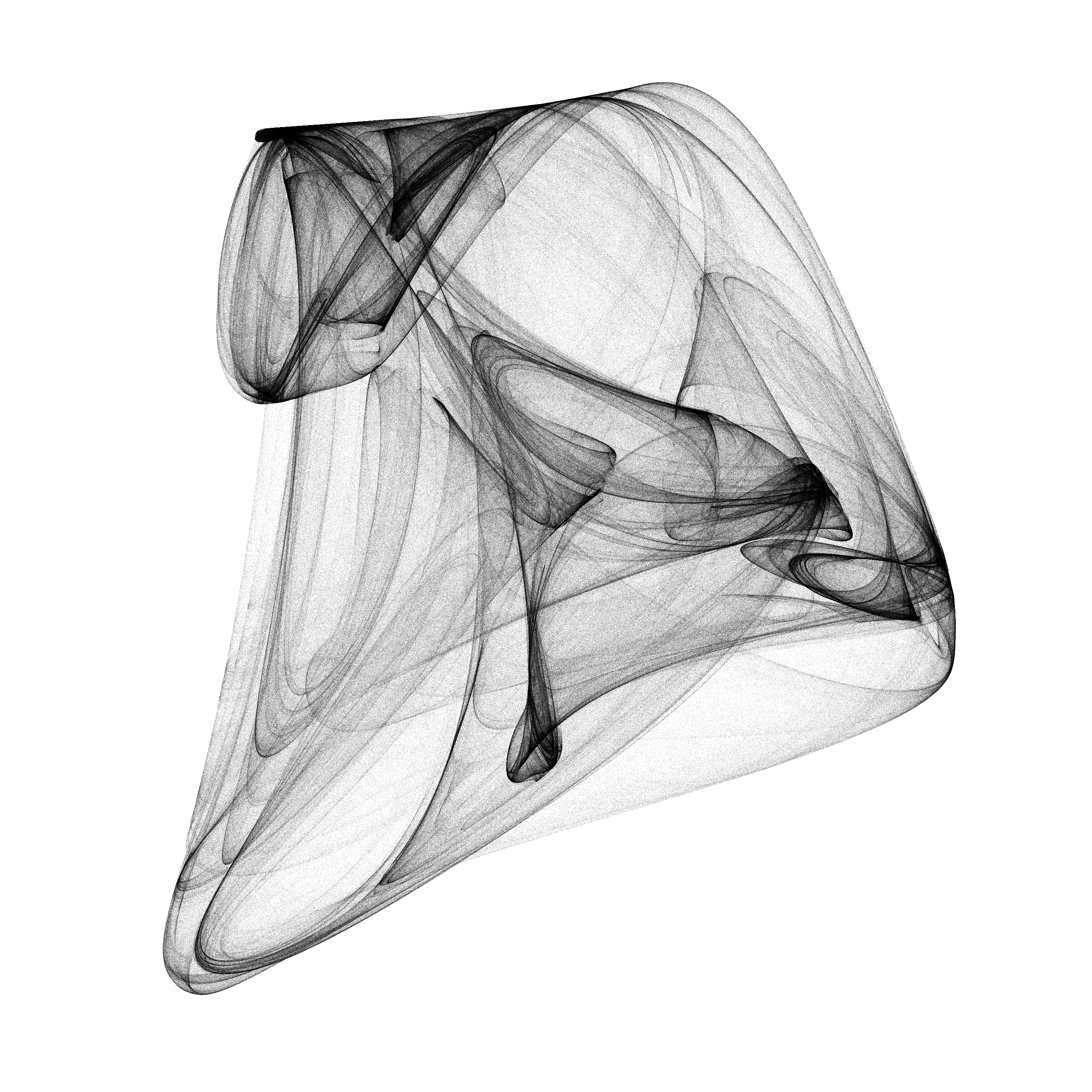
Now, here is a different set of equations with longer terms, but also just two control parameters:

\[x_{n+1} = \sin\left(y_n^2 + \varrho_n\,\sin(x_n + y_n)\right) + \cos(x_n - a\,y_n)\] \[y_{n+1} = \cos\left(x_n^2 + \varrho_n\,\sin(x_n + y_n)\right) + \sin(x_n - a\,y_n)\] \[\varrho_{n+1} = b\,\sin(x_n\,y_n)\]

With \(a = 0.5 \,\land\, b = 0.9\):

---

1. C.A. Pickover, 1988. "A Note On Rendering 3-D Strange-Attractors". Computers & Graphics. 12(2). doi:10.1016/0097-8493(88)90038-6 ↩

2. C.A. Pickover, 1990. "Computers, Pattern, Chaos, and Beauty". St. Martin’s Press. ISBN: 0312041233. ↩